我不确定您在这里找什么。通常通过功率谱密度或等效的自相关函数来描述噪声。随机过程的自相关函数及其PSD是傅立叶变换对。例如,白噪声具有脉冲自相关。这将在傅立叶域中转换为平坦的功率谱。
您的示例(而有些不切实际)是类似于在的载波频率观察载波调制的白噪声的通信接收机2ω。示例接收机非常幸运,因为它的振荡器与发射机的振荡器相干。在调制器和解调器产生的正弦波之间没有相位偏移,从而允许“完美”下变频至基带。单靠这并不是不切实际的。相干通信接收机的结构很多。但是,通常将噪声建模为通信信道的附加元素,该元素与接收器试图恢复的调制信号无关。发射机很少实际发送噪声作为其调制输出信号的一部分。
不过,通过这种方式,看看示例背后的数学可以解释您的观察。为了获得您描述的结果(至少在原始问题中如此),调制器和解调器均具有在相同参考频率和相位下工作的振荡器。调制器输出以下内容:
n(t)x(t)∼N(0,σ2)=n(t)sin(2ωt)
接收器生成下变频的I和Q信号,如下所示:
I(t)Q(t)=x(t)sin(2ωt)=n(t)sin2(2ωt)=x(t)cos(2ωt)=n(t)sin(2ωt)cos(2ωt)
一些三角恒等式可以使和Q (t )充实I(t)Q(t):
sin2(2ωt)sin(2ωt)cos(2ωt)=1−cos(4ωt)2=sin(4ωt)+sin(0)2=12sin(4ωt)
Now we can rewrite the downconverted signal pair as:
I(t)Q(t)=n(t)1−cos(4ωt)2=12n(t)sin(4ωt)
The input noise is zero-mean, so I(t) and Q(t) are also zero-mean. This means that their variances are:
σ2I(t)σ2Q(t)=E(I2(t))=E(n2(t)[1−cos(4ωt)2]2)=E(n2(t))E([1−cos(4ωt)2]2)=E(Q2(t))=E(n2(t)sin2(4ωt))=E(n2(t))E(sin2(4ωt))
You noted the ratio between the variances of I(t) and Q(t) in your question. It can be simplified to:
σ2I(t)σ2Q(t)=E([1−cos(4ωt)2]2)E(sin2(4ωt))
The expectations are taken over the random process n(t) 's time variable t. Since the functions are deterministic and periodic, this is really just equivalent to the mean-squared value of each sinusoidal function over one period; for the values shown here, you get a ratio of 3–√, as you noted. The fact that you get more noise power in the I channel is an artifact of noise being modulated coherently (i.e. in phase) with the demodulator's own sinusoidal reference. Based on the underlying mathematics, this result is to be expected. As I stated before, however, this type of situation is not typical.
Although you didn't directly ask about it, I wanted to note that this type of operation (modulation by a sinusoidal carrier followed by demodulation of an identical or nearly-identical reproduction of the carrier) is a fundamental building block in communication systems. A real communication receiver, however, would include an additional step after the carrier demodulation: a lowpass filter to remove the I and Q signal components at frequency 4ω. If we eliminate the double-carrier-frequency components, the ratio of I energy to Q energy looks like:
σ2I(t)σ2Q(t)=E((12)2)E(0)=∞
This is the goal of a coherent quadrature modulation receiver: signal that is placed in the in-phase (I) channel is carried into the receiver's I signal with no leakage into the quadrature (Q) signal.
Edit: I wanted to address your comments below. For a quadrature receiver, the carrier frequency would in most cases be at the center of the transmitted signal bandwidth, so instead of being bandlimited to the carrier frequency ω , a typical communications signal would be bandpass over the interval [ω−B2,ω+B2], where B is its modulated bandwidth. A quadrature receiver aims to downconvert the signal to baseband as an initial step; this can be done by treating the I and Q channels as the real and imaginary components of a complex-valued signal for subsequent analysis steps.
With regard to your comment on the second-order statistics of the cyclostationary x(t), you have an error. The cyclostationary nature of the signal is captured in its autocorrelation function. Let the function be R(t,τ):
R(t,τ)=E(x(t)x(t−τ))
R(t,τ)=E(n(t)n(t−τ)sin(2ωt)sin(2ω(t−τ)))
R(t,τ)=E(n(t)n(t−τ))sin(2ωt)sin(2ω(t−τ))
Because of the whiteness of the original noise process n(t), the expectation (and therefore the entire right-hand side of the equation) is zero for all nonzero values of τ.
R(t,τ)=σ2δ(τ)sin2(2ωt)
The autocorrelation is no longer just a simple impulse at zero lag; instead, it is time-variant and periodic because of the sinusoidal scaling factor. This causes the phenomenon that you originally observed, in that there are periods of "high variance" in x(t) and other periods where the variance is lower. The "high variance" periods are selected by demodulating by a sinusoid that is coherent with the one used to modulate it, which stands to reason.